WRF diaries
This is my personal notebook to help me run WRF
Installing WPS and WRF environment.
I have already done this part, so I’ll write a page on this some other day if I need to reinstall it. Meanwhile, here’s a much more sophisticated link for How to compile WRF from UCAR’s experts.
Part 1: WPS
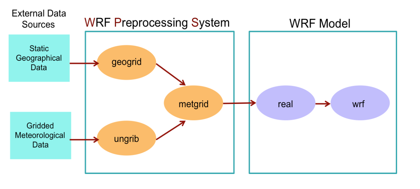
There are essentially three main steps to running the WRF Preprocessing System:
- Define a model coarse domain and any nested domains with
geogrid.exe - Extract meteorological fields from GRIB data sets for the simulation period with
ungrib.exe - Horizontally interpolate meteorological fields to the model domains with
metgrid.exe
Here, I have listed ungrib.exe workflow first, and then geogrid.exe. These are parallel processes and the order doesn’t matter.
Step 1a: Gridded Meteorological Data
- Choosing the Reanalysis dataset: List of available GRIB datasets from NCAR.
- In Google Earth Engine, I usually use the NCEP/NCAR Reanalysis dataset to visualize air temperatures. But its resolution is 209 km, not the best for intra-urban applications.
- Mostly they use NCEP FNL (Final). Resolution 1 degree.
- For USA, NCEP North American Mesoscale (NAM) with 12 km 6 hourly outputs (Vtable:
Vtable.NAM) might be better. (Will update when I run USA case studies) - For New Delhi, I used NCEP GDAS/FNL 0.25 Degree.
- V-table called
Vtable.GFSshould be used and can be found here.
- V-table called
- For Paris, I used ERA by ECMWF.
- ERA-interim has GRIB files.
- ERA5 Reanalysis has NetCDF outputs only.
- The prescribed V-table called
Vtable.ERA-interim_plcan be found here.
- Finding the right ERA-interim Reanalysis files (Sign in required):
- Last time, I made the mistake of downloading NetCDF formats of ERA5 and ran into an error where it showed 0 available levels of soil depth. However,
WRF/ungribis not yet adapted to handle netCDF files. Be sure to download GRIB files. - Use the “Web Server Holding” column to access the whole files, not the “Data Format Conversion” column.
- For atmospheric variables: Use the “ERA Interim atmospheric model analysis interpolated to pressure levels” group for WRF, not the “ERA Interim atmospheric model analysis on model levels” group.
- For surface variables: Use “ERA Interim atmospheric model analysis for surface” group.
- Last time, I made the mistake of downloading NetCDF formats of ERA5 and ran into an error where it showed 0 available levels of soil depth. However,
- Downloading the files.
- Pick “Faceted Browse” and enter the time period of interest. The files are huge (over 100 MB each) so only download the time period needed.
- Use download option 2 that generates a Unix script to read them all using wget.
- Copy the contents and paste them in a new file created in
$RCAC_SCRATCHusingvi <name_of_script>. Within the file, update the NCAR password. - Make the file executable using
chmod 755 <name_of_script>. Although mine worked regardless. - Note that this is a
.cshscript so run it usingcsh Wget-City-atm.shbut save it as.shnonetheless. When I create a.cshtype file, the text gets pasted with a#comment sign in front of every line. Then move the downloaded files to a separate folder andpwdthe location for next step. - Possible wget error:
HTTP request sent, awaiting response... 403 Forbidden. Solution: Sign out of NCAR website and sign in again and accept the new terms and conditions.
Step 1b: UNGRIB.
-
Translating the ERA-interim GRIB files into intermediate file format the MetGrid will read. Note that it does NOT cut down the data according to the domain specification yet.
- Link the Vtable using
ln -sf ungrib/Variable_Tables/<name_of_Vtable> VtableExecute these steps within the folderBuild_WRF/WPS/. -
Link the location of downloaded data using
./link_grib.csh <path_to_data> .(here)NOTE: Make sure to link the files, not just the folder. There is no need to put a ‘*’ following the directory in the above command. The script will automatically grab all of the files beginning with the given prefix. This step should create several links of the formatGRIBFILE.AAA. - Edit the
&sharepart of namelist.wps file. The current run specifications should always be stored asnamelist.wps(inBuild_WRF/WPS/). Therefore, backup the original and keep renaming the completed runs.&sharestart_dateandend_date: three times for each domain. Avoid this error - Check to make sure you have an underscore _ between the day and hour in the dates in yournamelist.wpsand not a dash - .interval_seconds = 21600(for 6 hourly ERA data).- leave
io_form_geogrid = 2for NetCDF as ungrib will convert our reanalysis data to netcdf.
&ungribprefix: Leave it at the default option,FILE.
- Run
./ungrib.exeto generate intermediate files in the format ofFILE:YYYY-MM-DD_hh- one file for each time. - If there are any errors,
vi ungrid.logto check what errors.Shift+Gwill take you to the last line.
Step 2a: Static Geographical Data.
-
Download and save the highest resolution as well as the lowest resolution of each field from here - Geographical Input Data Mandatory Fields Downloads - using
wgetand save it in$RCAC_SCRATCH. -
Unlike meteorological data, there is no need to download Geographic data every time because this is just static.
-
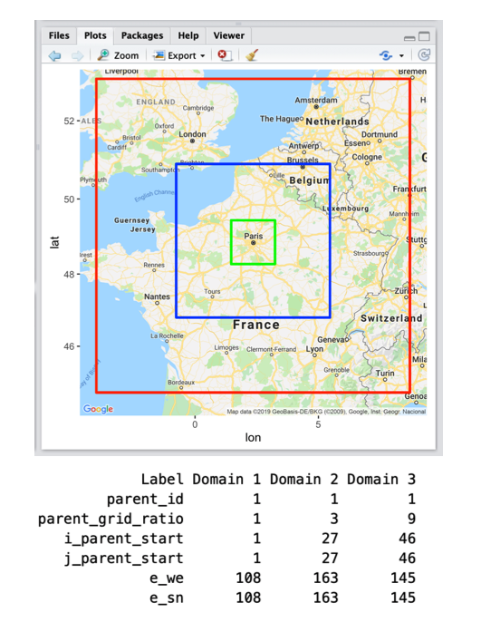
Use the R script to visualize and configure domains. Note: It is recommended to have domains no smaller than about 100x100 each. Keep about 10 grid points (minimum of 5) on each side, in the boundary zone. If domains are too small, the solution will be determined by forcing data.
Step 2b: GEOGRID.
- Edit the
&geogridpart of namelist.wps file.&geogrid- Input from R domain designer.
geog_data_res: Possible resolutions include ’30s’, ‘2m’, ‘5m’, and ‘10m’, where ‘s’ is arc-second and ‘m’ is arc-minute.- Using
geog_data_res = '5m','2m','30s'threw this error:ERROR: Could not open /RCAC_SCRATCH/DATA/WPS_GEOG/soiltype_top_2m/index application called MPI_Abort(MPI_COMM_WORLD, 0) - process 0. geog_data_res = '5m','5m','30s',works.- used
nlcd2011_ll_9s+urbfrac_nlcd2011+30sfor NLCD.
- Using
dx and dy = 9000. Resolution of largest domain (in meters for Lambert and Mercator projection. Degrees in Lat-Lon projection).map_proj = 'Lambert'for mid-latitude European countries. Mercator will probably be better for India. [1=Lambert, 2=polar stereographic, 3=mercator, 6=lat-lon]ref_latandref_lonare the center of largest domain. Usegeocode(City)in R.truelat1 = ref_latrequired for Lambert, map_proj = 1, 2, 3 (defaults to 0 otherwise).truelat2- required for MAP_PROJ = 6 (defaults to 0 otherwise).stand_lon = ref_lon: If this longitude is set to the same value as ref_lon, your largest domain will be centered.geog_data_path: Location of Geographical datasetWPS_GEOGin RCAC_SCRATCH.
-
Load ncl –
module load nclThen runncl util/plotgrids_new.nclto make sure geogrid is in order. - Run
./geogrid.exeto generate intermediate files in the format ofgeo_em.dxx.nc- one file for each domain saved in the WPS folder.
Step 3: METGRID.
- Add the line
opt_output_from_metgrid_path = RCAC_SCRATCH/METGRID_FILES/in the&metgridsection. - Run
./metgrid.exe - (Optional) Make sure
METGRID.TBLis linked correctly toMETGRID.TBL.ARWusingls metgrid/METGRID.TBL. This is also true for the other three programs. - This will generate netCDF outputs of the format
met_em.dxx.YYYY-MM-DD_hh:00:00.nc- one file per time per domain.- This step was generating empty files (and yet it displays the success message). Turns out I didn’t have enough space in my home drive. But this can be easily fixed by saving the outputs to the Scratch drive.
- For LA, ran into this error.
Part 2: WRF.
Step 4: Setup namelist.input
- Edit the namelist.input file in the
WRF/run/folder. (Here’s a list of what I used for Paris run)&time_control- No need to specify number of days and hours. Set those to 0. Set start and end dates.
interval_seconds = 21600: the time interval of Reanalysis dataset.input_from_file = .true.: Setting this to .true. for nested domains will allow the real.exe program to createwrfinput_d0*files for the nested domains.history_interval = 60: frequency of output files in minutes (set to hourly)history_outname = $RCAC_SCRATCH/WRFOUTS/<City_name>/wrfout_d<domain>_<date>(personal convention). This is an optional feature to save the outputs in another directory.frames_per_outfile: Number of hourly output files to be combined in one. Set it to 1000 to set upto 40 days worth of output into a single file.restart_interval = 1440: Backing up every X minute to restart run from that point if WRF crashes. Ideally keep it at 6 hours (360), maybe 1 day (1440) for long runs.- Keep
io_form_* = 2for NEtCDF formats.
&domainstime_step = 45: Time step (in seconds) for integration. This should be kept low. About 5 to 6 times the grid size of largest domain, i.e. 45 seconds for 9 km cases.- But I ran into CFL error with 45 seconds. They typically indicate that the model is becoming unstable. The first thing to do in such a case is to rerun the model with a reduced time step. Reduce
time_step = 36seconds.
- But I ran into CFL error with 45 seconds. They typically indicate that the model is becoming unstable. The first thing to do in such a case is to rerun the model with a reduced time step. Reduce
parent_time_step_ratio = 1, 3, 9,scales the time step as well for each domain.e_snande_we: same asnamelist.wps.e_vert: Vertical levels. It is not recommended to have fewer than 35 levels. Typically 40-60 levels is recommended. For NYC July 2006 heat wave, 60 were used.p_top_requested = 5000: Default value for the pressure top (in Pa) to use in the model.- **Now use the command
ncdump -h met_em.d01.<date>in the folder withmet_emfiles to find out the values of the following variables.num_metgrid_levels(near top)num_metgrid_soil_levels(near bottom)**
- ` parent_time_step_ratio = 1, 3, 9,
same as theparent_grid_ratio`. feedack = 1andsmooth_option = 0for updating the parent domain based on nested domains.
&physics- Detailed descriptions here. Options recommended for 1 – 4 km grid distances, convection-permitting runs for a 1- 3 day run (as used for the NCAR spring real-time convection forecast over the US in 2013) are noted as “NCAR recommended”.physics_suite =Set to either CONUS or Tropical tunes the remaining parameters to a saved setting. Delete this option.mp_physics = 8,8,8,- 8 = New Thompson et al. scheme: A new scheme suitable for high-resolution simulations (NCAR recommended)
cu_physics = 2,0,0,- 0 = Not used, because at a high resolution of 1-4 km, we can explicitly resolve the cumulus clouds, no need to parameterize them.
- 1 = Kain-Fritsch scheme.
- 2 = Betts-Miller-Janjic scheme.
ra_lw_physics = 1,1,1,- 1 = Rapid Radiative Transfer Model (RRTM) used in NYC 2006 run.
- 4 = Updated RRTMG. (CONUS, NCAR recommended)
ra_sw_physics = 1,1,1,- 1 = Dudhia Scheme.
- 4 = RRTMG shortwave (CONUS, NCAR recommended)
bl_pbl_physics = 2,2,2,- 2 = Mellor-Yamada-Janjic (MYJ) scheme. (NYC, NCAR, CONUS default)
- 8 = Bougeault and Lacarrere (BouLac) PBL scheme. (Designed for use with BEP urban model.)
sf_sfclay_physics = 2,2,2,- 2 = Eta similarity: Based on Monin-Obukhov with Zilitinkevich thermal roughness length (NYC 2006, NCAR recommended).
sf_surface_physics = 2,2,2,- 2 = Noah Land Surface Model (CONUS)
- 4 = Noah-MP (multi-physics) Land Surface Model
- 5 = Community Land Model (CLM)
radt = 10,10,10: minutes between radiation physics calls. Recommended 1 minute per km of dx (e.g. 10 for 9 km grid); use the same value for all nests.bldt = 0: minutes between boundary-layer physics calls (0=call every time step)cudt = 0: minutes between cumulus physics calls. This should be set to 0 when using all cu_physics except Kain-Fritsch (cu_physics = 1).icloud = 1: use Xu-Randall methodnum_land_cat: Number of Land categories in input dataset- 24 = USGS (pre V3.8 default)
- 20 = MODIS
- 28 = USGS including lake category
- 21 = MODIS (post V3.8 default)
- 40 = NLCD (CONUS only)
sf_urban_physics = 2- 1 = single layer Urban Canopy Model (UCM),
- 2 = Multi-layer, Building Environment Parameterization (BEP) scheme (works only with
sf_surface_physics = 2(Noah LSM) andbl_pbl_physics = 2 or 8(MYJ or BouLac PBL). - 3 = Building Energy Model (BEM)
&dynamicskm_opt= 4- 3 = Smagorinsky 3d deformation (NYC).
- 4 = 2d deformation
- Don’t modify anything else.
Step 5: Run Real.exe
- Within the
WRF/run/folder, link themet_emfiles generated usingln -sf RCAC_SCRATCH/METGRID_FILES/met_em.d0* .(here) - Run
./real.exe- For Paris, ran into this error. Solution is listed in the known problems list under ERA-Interim data problem –> In the section
&physics, add the linesurface_input_source = 1to overwrite the default value of 3. - For LA, ran into NLCD error. Downloading NLCD urban fraction dataset for CONUS from here.
- This creates
wrfbdy_d01,wrfinput_d01,wrfinput_d02, andwrfinput_d03files. Along withnamelist.output,rsl.outandrsl.errorfiles, which will clearly specify the error, or say “SUCCESS COMPLETE REAL_EM INIT” if they are no errors. - NOTE: Print out the sizes of all rsl.error files to check which has the most information. The error files are not all the same. Only the largest one contains most relevant information about a failure (if any).
- For Paris, ran into this error. Solution is listed in the known problems list under ERA-Interim data problem –> In the section
Step 6: Submit WRF run
- Use
qlistto find out how many nodes are available in each queue. - We wrote a script called
WRF/run/qsubmit.shto submit WRF runs to Halstead clusters.#!/bin/sh -l: Specifying the format# FILENAME: uhi: Commented description of run.#PBS -q <q_name>: Chosen queue#PBS -l nodes=5:ppn=20: In Halstead every node contains 20 processor per node (ppn). So, we select 5 nodes of 20 ppn each.#PBS -l walltime=72:00:00: Time after which Halstead will kill our process.#PBS -N PARIS: Job Name.mpiexec -n 100 <path_to_WRF>/run/wrf.exe: Command with address to execute it.
- Run the script using
qsub <path_to_file>/qsubmit.sh - Use
qstat -u $USERto check status. - Remember to run
./real.exeagain if you modify anything innamelist.inputbefore submitting WRF run again.